Notes

A place to record somethings related to programming.


  • 首頁

  • 歸檔

  • 標籤

  • 檢索

Machine learning note

發表於 2015-02-24 |

https://class.coursera.org/ml-008/

Supervised Learning:

Right answers are given.

Regression problem:
Predict continuous value output.

Classification problem:
Discrete value output.

Unsupervised Learning:
Correct answers are not given to computer. Find the structure in the data.

Linear Regression with One Variable:
ax+b = y minimize the squared error with training data.

Gradient Descent:
Using the different value initialization will lead to different optimal result.( \theta_j := \theta_j - \alpha \frac{\partial }{\partial \theta_j}J(\theta_0, \theta_1) )
(\alpha) is called learning rate. It controls how big a step we take downhill to gradient descent.
If the alpha is too small, gradient descent can be slow.
If the alpha is too large, it may fail to converge, or even diverge.
Simultaneous update ( \theta_0, \theta_1 ).
In linear regression, the cost function is a convex function (bowl-shape function). So the gradient descent can find the only global optimum.
If the cost function is not convex, then gradient descent may find any local optima.

Linear Regression with Multiple Variable:
( h_{\theta}(x) = \theta_0+\theta_1 x_1+\theta_2 x_2+…+\theta_n x_n )
For convenience, ( x0 = 1 )
( J(\theta) = \frac{1}{2m} \sum
{i=1}^m{(h_{\theta}(x^{(i)}) - y^{(i)})^2} )
Use gradient descent: ( \theta_j = \thetaj - \alpha \frac{1}{m} \sum{i=1}^m{(h_{\theta}(x^{(i)}) - y^{(i)}) x_j^{(i)}} )
Feature scaling
For gradient descent, we need to do feature scaling to make features in the range -3<value<3. All features in the similar range can make gradient descent more quickly.
In general, feature scaling is: ( x = \frac{x-mean}{standard \, deviations} )
And in practice, in training stage, we should save every feature’s mean and standard deviation. Because in predict stage, we still need to do the feature scaling first.
Learning rate
The learning rate ( \alpha ):
If ( \alpha ) is too small: slow convergence.
If ( \alpha ) is too large: ( J(\theta) ) may not decrease on every iteration and may not converge.
In practice, we can try learning rate in log scale which is about 3 times the previous value (ie., 0.3, 0.1, 0.03, 0.01 and so on).
Feature selecting and polynomial regression
Besides, we can do some features selecting and polynomial regression in linear regression.
For example, we can multiply two features to create new feature or omit some features.
Polynomial regression example: ( \theta_0 + \theta_1 x + \theta_2 x^2 + \theta_3 x^3 )
If the x is the feature: “size”. ( x_1 = (size) \quad x_2 = (size)^2 \quad x_3 = (size)^3 )
Normal equation
In addition to gradient descent, we can use normal equation to solve linear regression ( \theta ) analytically.
So in general, We do differentiation in cost function ( J(\theta) ) for every ( \theta ) and set it to zero. In order to find the minimum value of the cost function.
And actually we can directly do it in matrix in linear regression. We want ( X \theta = y ), therefore ( \theta = (X^\top X)^{-1} X^\top y ).
In summary, normal equation’s advantages are:
1. No need to choose ( \alpha )
2. Don’t need to iterate
The disadvantages are:
1. Need to compute ( (X^\top X)^{-1} )
2. Slow if the number of feature(n) is very large(>10000).

Logistic Regression
In classification problem, the linear regression is not a good method to solve it. We can use the logistic regression to solve classification problem. (Define a new Hypothesis and cost function.)
The hypothesis in linear regression is: ( h_{\theta}(x) = \theta_0+\theta_1 x_1+\theta_2 x_2+…+\theta_n xn = \theta^\top x )
The new hypothesis in logistic regression is: ( h
\theta(x) = g(\theta^\top x) = \frac{1}{1+e^{-\theta^\top x}} ) which g is a sigmoid function.
And it actually represent the possibility that y=1 on input x.

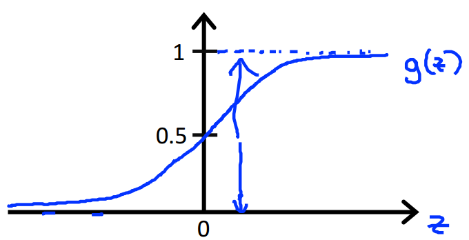
So based on the hypothesis, we will predict y=1 if ( J(\theta) ) >= 0.5. In other word, when ( \theta^\top x ) >= 0.
And that is called decision boundary.

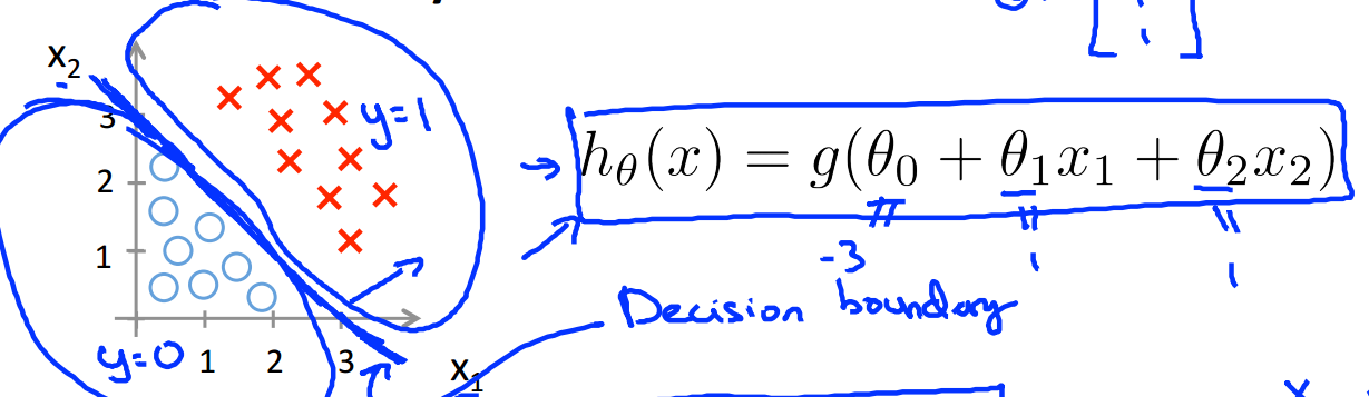
The decision boundary can be non-linear when we use other function in ( \theta^\top x ) just like in linear regression.

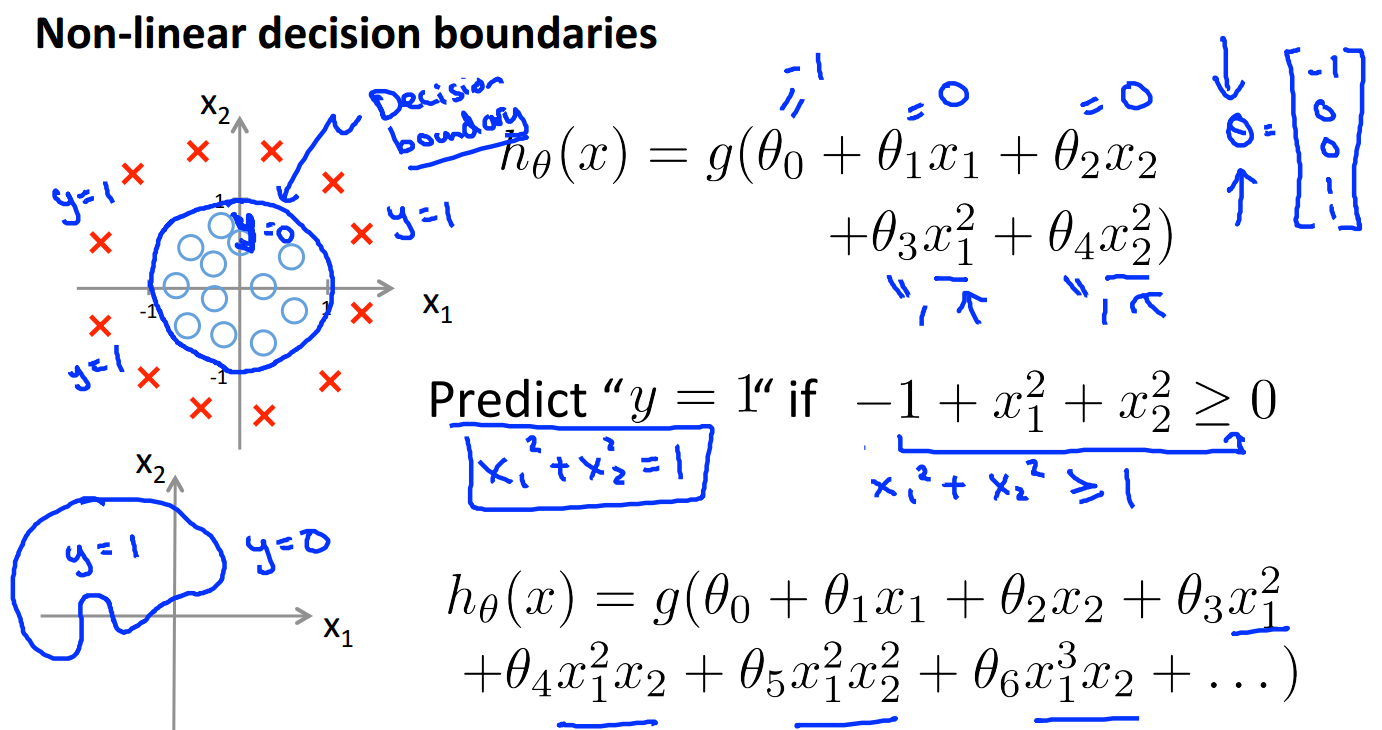
Then in cost function.
The cost function in linear regression is: ( J(\theta) = \frac{1}{2m} \sum{i=1}^m{(h{\theta}(x^{(i)}) - y^{(i)})^2} )
We cannot use it in logistic regression because the (h_\theta(x)) is change. And it contain a sigmoid function that it produces a non-convex function when we use this cost function.
Therefore, we change the function inside the summation to:

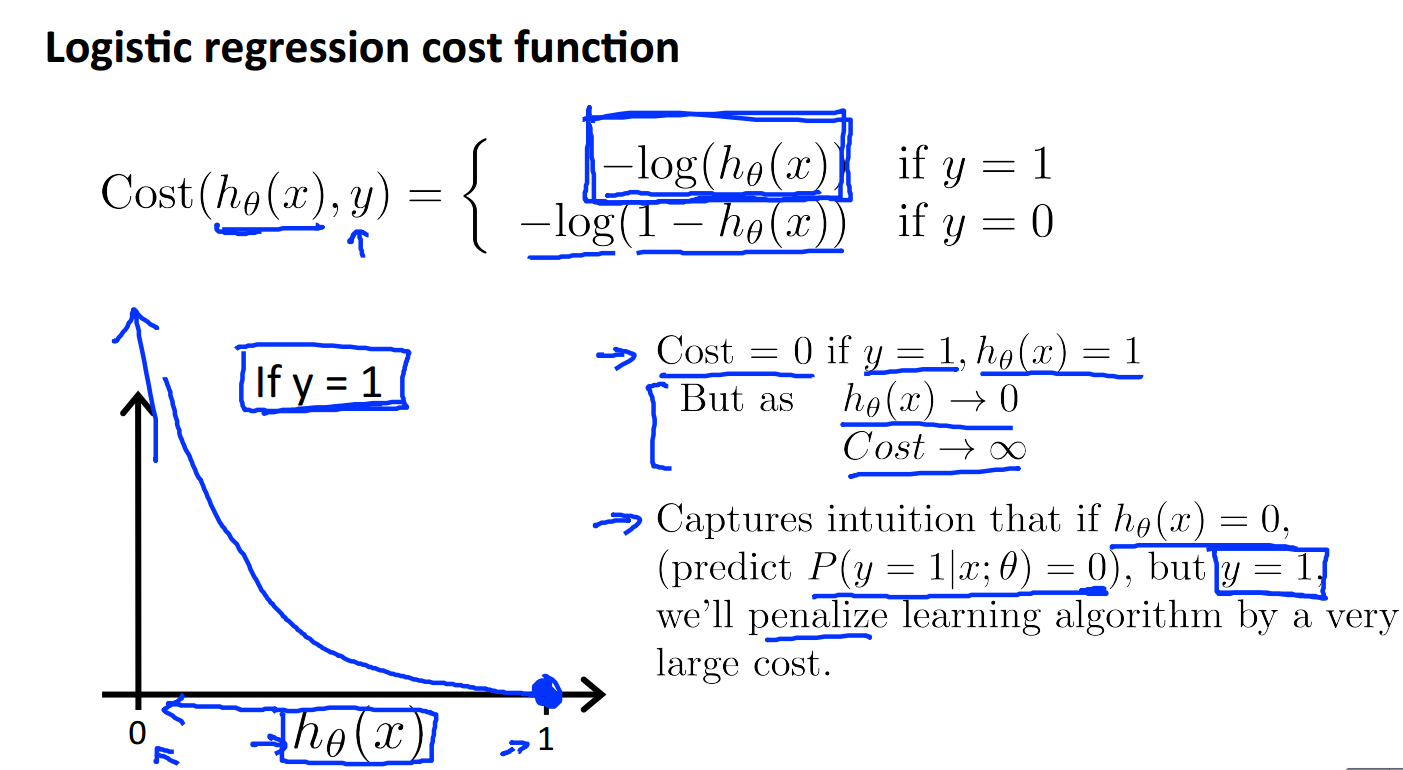
Because we use it in binary classification, and y=0 or 1, so can simplified it to: ( -ylog(h\theta(x))-(1-y)log(1-h\theta(x)) )
Finally the cost function is: ( J(\theta) = -\frac{1}{m}[\sum{i=1}^m{ y^{(i)} log(h\theta(x^{(i)})) + (1-y^{(i)}) log(1-h_\theta(x^{(i)})) }] )
And it is derived from statistics using the principle of maximum likelihood estimation. It also has a nice property that it is convex.
Now we have cost function, we can use it to do gradient descent to find the minimum cost. Same as in linear regression, the gradient descent is:
( \theta_j = \theta_j - \alpha \frac{\partial}{\partial\theta_j} J(\theta) )
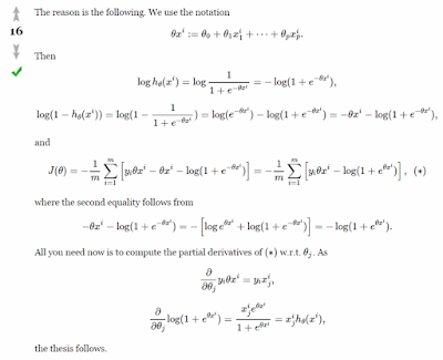
After differential the cost function, we can get:
( \theta_j = \thetaj - \alpha \frac{1}{m} \sum{i=1}^m{(h_{\theta}(x^{(i)}) - y^{(i)}) xj^{(i)}} )
In surprise, it’s totally same as the gradient descent in linear regression.
The way to differential the cost function is show in below by picture.
http://math.stackexchange.com/questions/477207/derivative-of-cost-function-for-logistic-regression
[![](https://3.bp.blogspot.com/-kXLqV5SwoL4/VOtaMF-UGdI/AAAAAAAAANc/M8SEcFVYgo4/s400/FireShot%2BCapture%2B-%2Bstatistics%2B-%2Bderivative%2Bof%2Bcost%2Bfunctio
%2B-%2Bhttp_math.stackexchange.comquesti.png)](http://3.bp.blogspot.com/-kXLqV5SwoL4/VOtaMF-UGdI/AAAAAAAAANc/M8SEcFVYgo4/s1600/FireShot%2BCapture%2B-%2Bstatistics%2B-%2Bderivative%2Bof%2Bcost%2Bfunctio%2B-%2Bhttp_math.stackexchange.com_questi.png)
We can do gradient descent by vectorization in matlab:

In addition to gradient descent, there are other way to optimize the cost function. Like Conjugate gradient, BFGS, L-BFGS. The advantages are no need to select ( \alpha ) rate and more fast. But disadvantage is more complex.
However, we can use them easily by matlab without knowing any about their actually algorithm.
What we need to do in matlab is writing the function return cost and the partial derivatives value when given theta. And matlab will chose the appropriate method for us.
For example, the function we should write in the format like:

function [jVal, gradient] = costFunction(theta)
jVal = (theta(1)-5)^2 + (theta(2)-5)^2;
gradient = zeros(2,1);
gradient(1) = 2(theta(1)-5);
gradient(2) = 2
(theta(2)-5);
And use it by:

options = optimset(‘GradObj’, ‘on’, ‘MaxIter’, ‘100’);
initialTheta = zeros(2,1);
[optTheta, functionVal, exitFlag] = fminunc(@costFunction, initialTheta, options);
The optTheta will be the optimization theta.
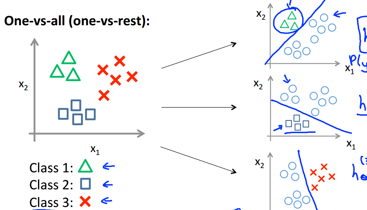
Besides, we can also use logistic regression in multi-calss classification.
The way is just train a logistic regression classifier for each class. And pick the class that probability is maximum as the result.

Alternative to TestFlight?

發表於 2015-02-23 |

https://www.linkedin.com/groups/Alternative-TestFlight-712237.S.5968340843382194176?view=&item=5968340843382194176&type=member&gid=712237&trk=eml-b2_anet_digest-group_discussions-10-grouppost-disc-3&midToken=AQF2z_g07q8BBw&fromEmail=fromEmail&ut=0RIXkGlrlEkmE1 Try Crashlytics!

Python pyenv and virtualenv usage note

發表於 2015-02-09 |

Installation:


pyenv


Mac


brew update
brew install pyenv

To upgrade pyenv in the future, just use upgrade instead of install.

After installation, you’ll still need to add eval “$(pyenv init -)” to your profile (add it to ~/.bash_profile). You’ll only ever have to do this once.

#### Others

# Get Code
git clone https://github.com/yyuu/pyenv.git ~/.pyenv

# Set the Paths
echo ‘export PYENV_ROOT=”$HOME/.pyenv”‘ >> ~/.bash_profile
echo ‘export PATH=”$PYENV_ROOT/bin:$PATH”‘ >> ~/.bash_profile
Zsh note: Modify your ~/.zshenv file instead of ~/.bash_profile.
Ubuntu note: Modify your ~/.bashrc file instead of ~/.bash_profile.

# Initialize pyenv on load of terminal
echo ‘eval “$(pyenv init -)”‘ >> ~/.bash_profile
exec $SHELL

### pyenv-virtualenv

Mac


brew install pyenv-virtualenv

Add
eval “$(pyenv virtualenv-init -)”
to your profile (add it to ~/.bash_profile)

Others


# Install pyenv virtualenv
git clone https://github.com/yyuu/pyenv-virtualenv.git ~/.pyenv/plugins/pyenv-virtualenv

# auto ativate virtualenv for pyenv
echo ‘eval “$(pyenv virtualenv-init -)”‘ >> ~/.bash_profile
Zsh note: Modify your ~/.zshenv file instead of ~/.bash_profile.
Ubuntu note: Modify your ~/.bashrc file instead of ~/.bash_profile.
# restart shell
exec $SHELL

Usage


pyenv


# install python
pyenv install 2.7.9
pyenv install 3.4.3

if there are problems when install the python, you can refer to

# https://github.com/yyuu/pyenv/wiki/Common-build-problems

rehash when install the new versions every time

pyenv rehash

set version of python to use for this session

pyenv shell 3.4.3

set global python for everytime we start pyenv

pyenv global 3.4.3

set python version for current and all sub directories

pyenv local 3.4.3

pyenv-virtualenv


Restart the shell and let’s create an virtualenv with Python 2.7.8.
pyenv virtualenv 2.7.8 project-a-2.7.8

Activate the newly created virtualenv.
pyenv activate project-a-2.7.8

You can deactivate the current virtualenv.
pyenv deactivate

And list the available virtualenvs.
pyenv virtualenvs

Those virtualenvs are located in ~/.pyenv/versions just like those installed Pythons. If you want to remove a virtualenv, simply delete that corresponding folder.
Or
pyenv uninstall my-virtual-env

Reference:
http://eureka.ykyuen.info/2014/07/11/pyenv-python-version-manager/
http://eureka.ykyuen.info/2014/07/14/manage-your-python-projects-with-virtualenv/
http://blog.froehlichundfrei.de/2014/11/30/my-transition-to-python3-and-pyenv-goodby-virtualenvwrapper.html
https://godjango.com/96-django-and-python-3-how-to-setup-pyenv-for-multiple-pythons/
https://github.com/yyuu/pyenv
https://github.com/yyuu/pyenv-virtualenv
http://www.openfoundry.org/tw/tech-column/8516-pythons-virtual-environment-and-multi-version-programming-tools-virtualenv-and-pythonbrew

Imgae alignment

發表於 2015-02-07 |

Newton’s method:

Find the f(x) = 0.
For an initialized point, calculate the tangent line. And set the point that is intersection of x-axis and tangent line as next x.
As the animated picture from wiki:

So write in math:
( x_{n+1} = x_n - \frac{f(x_n)}{f^\prime(x_n)} )

Lucas-Kanade:

When in image alignment that only translation:
( E(u, v) = \sum{x,y}{(I(x+u, y+v) - T(x, y))}^2 )
Do Taylor’s expand in I(x+y, y+v):
( E(u, v) = \sum
{x,y}{(I(x, y) - T(x, y) + uI_x + + vIy)}^2 )
And differentiate to find the extremal point:
( 0 = \frac{\partial E}{\partial u} = \sum
{x,y}{2I_x(I(x,y)-T(x,y)+uI_x+vIy)} )
( 0 = \frac{\partial E}{\partial v} = \sum
{x,y}{2I_y(I(x,y)-T(x,y)+uI_x+vIy)} )
Reformat as matrix:
( \begin{bmatrix} \sum
{x,y}{Ix^2} & \sum{x,y}{I_xIy} \ \sum{x,y}{I_xIy} & \sum{x,y}{Iy^2} \end{bmatrix} \begin{bmatrix} u \ v \end{bmatrix} = \begin{bmatrix} \sum{x,y}{Ix(T(x,y)-I(x,y))} \ \sum{x,y}{I_y(T(x,y)-I(x,y))} \end{bmatrix} )
One thing to note:
Although in the math is plus u and v.
But if we write in transformation matrix, it is minus u and v.
Because I(x+u, y+v) means original x, y becomes the x-y, y-v in a transformed image.

circular convolution
1. why don’t just use translation matrix to fit
2. d/dx d/dy use which kernel is better

Postgres backup by pg_dump and psql restore

發表於 2015-02-05 |

pg_dump –data-only -t “\”MixedCaseName\”” > xxx.txt
(add -o if you want to retain id)

Use psql to delete all data from the table.

sudo sudo -u username psql -U username -d dbname -f filename(xxx.txt)

Running a Reverse Proxy in Apache

發表於 2015-01-22 |

ps -ef | grep apache
/usr/sbin/apache2 -V | grep SERVER_CONFIG_FILE

sudo a2enmod mod_proxy
sudo a2enmod proxy_http

In apache config file:
ProxyPass /app1/ http://internal1.example.com/
ProxyPassReverse /app1/ http://internal1.example.com/

service apache2 restart

Using openCV SIFT in C++

發表於 2015-01-19 |

1.

#include <opencv2\nonfree\features2d.hpp>
#include <opencv2\nonfree\nonfree.hpp>
2\. link opencv_nonfree247.lib (247 is your opencv version) 3\.
initModule_nonfree();

Ptr<cv::FeatureDetector> detector = FeatureDetector::create("SIFT"); 
Ptr<cv::DescriptorExtractor> descriptor = DescriptorExtractor::create("SIFT"); 

// detect keypoints
std::vector<KeyPoint> keypoints1;
detector->detect(img1, keypoints1);

// extract features
Mat desc1, desc2;
descriptor->compute(img1, keypoints1, desc1);

Linear Algebra

發表於 2014-12-18 |

( 2x-y = 0 )
( -x+2y = 3 )
Row picture: intersection of planes
( \begin{bmatrix} 2 & -1 \ -1 & 2 \end{bmatrix} \begin{bmatrix} x \ y \end{bmatrix} = \begin{bmatrix} 0 \ 3 \end{bmatrix} )
Column picture: combine vectors to produce right hand. Or called it as a linear combination of columns.
( x \begin{bmatrix} 2 \ -1 \end{bmatrix} + y \begin{bmatrix} -1 \ 2 \end{bmatrix} = \begin{bmatrix} 0 \ 3 \end{bmatrix} )
Ax = b have solution when A is invertible(non-singular case).
And we can say Ax is a combination of columns of A.

Elimination

Select the first row first column as pivot, and elimination all row below it, to make these row’s first columns become zero.
Then select the second row second column as pivot. elimination all row below it to make these row’s second columns become zero.
Do it recursive until reach the last row.

One thing to note is “pivots cannot be zero”

So the elimination fail when A matrix is singular matrix.
We can exchange the row’s positions to make pivots not zero when A matrix is not singular matrix.
( \begin{bmatrix} 0 & 1 \ 1 & 0 \end{bmatrix} \begin{bmatrix} 0 & 2 \ 3 & 1 \end{bmatrix} = \begin{bmatrix} 3 & 1 \ 0 & 2 \end{bmatrix} )
And we can express these operations in matrix form.
(When we put a matrix in the left of A, it is a combination of rows of A. Just like the above example to exchange row 1 and row 2.
When we put a matrix in the right of A, it is a combination of columns of A. Like the below example to exchange col 1 and col 2.)
( \begin{bmatrix} 0 & 2 & 1\ 3 & 1 & 2\ 1 & 2 & 3 \end{bmatrix} \begin{bmatrix} 0 & 1 & 0 \ 1 & 0 & 0 \ 0 & 0 & 1 \end{bmatrix} = \begin{bmatrix} 2 & 0 & 1 \ 1 & 3 & 2 \ 2 & 1 & 3 \end{bmatrix} )

Example for elimination:
( x+2y+z = 2 )
( 3x+8y+z = 12 )
( 4y+z = 2 )
( \begin{bmatrix} 1 & 0 & 0 \ 0 & 1 & 0 \ 0 & -2 & 1 \end{bmatrix} \begin{bmatrix} 1 & 0 & 0 \ -3 & 1 & 0 \ 0 & 0 & 1 \end{bmatrix} \begin{bmatrix} 1 & 2 & 1 \ 3 & 8 & 1 \ 0 & 4 & 1 \end{bmatrix} = \begin{bmatrix} 1 & 2 & 1 \ 0 & 2 & -2 \ 0 & 0 & 5 \end{bmatrix} )
It can be expressed as:
( E{32} E{21} A = U ) or just ( E A = U )
So do the same multiplication on b, we can get z value first. And back-substitution to get x and y.

Multiplication

Not commutative, but associative.
( AB = C )
( A=mn \qquad B=np \qquad C=m*p )

  1. Row times column( C{34} = (row\,3\,of\,A) \cdot (column\,4\,of\,B) = a{31}b{14} + a{32}b{24} + … = \sum\limits{k=1}^n a{3k}b{k4} )2. Column wayColumns of C are combinations of columns of A( \begin{bmatrix} \; & \; \end{bmatrix} \begin{bmatrix} | & | \end{bmatrix} = \begin{bmatrix} | & | \end{bmatrix} )3. Row wayRows of C are combinations of rows of B( \begin{bmatrix} - \end{bmatrix} \begin{bmatrix} \; \end{bmatrix} = \begin{bmatrix} - \end{bmatrix} )4. Column times rowSum of (cols of A) * (rows of B)( \begin{bmatrix} 2 & 7 \ 3 & 8 \ 4 & 9 \end{bmatrix} \begin{bmatrix} 1 & 6 \ 0 & 0 \end{bmatrix} = \begin{bmatrix} 2 \ 3 \ 4 \end{bmatrix} \begin{bmatrix} 1 & 6 \end{bmatrix} + \begin{bmatrix} 7 \ 8 \ 9 \end{bmatrix} \begin{bmatrix} 0 & 0 \end{bmatrix} )5. Block way( \begin{bmatrix} A_1 & A_2 \ A_3 & A_4 \end{bmatrix} \begin{bmatrix} B_1 & B_2 \ B_3 & B_4 \end{bmatrix} = \begin{bmatrix} A_1B_1+A_2B3 & \ \ _ & _ \end{bmatrix} )

Inverses of square matrices

( A^{-1}A = I = AA^{-1} )
Only when matrix is square, we can put inverse of A after A to get I. (A must to be square to be invertible?)
But not all matrices have inverses. An inverse is impossible when Ax is zero and x is non zero.
Because ( A^{-1}Ax = A^{-1}0 ) means ( Ix = A^{-1}0 ) means ( x = 0 ). So it is impossible to find inverse of A when x is nonzero and there exist Ax is zero.
The inverse exists if and only if elimination produces n pivots

Gauss-Jordan method to compute inverse of A
Put the matrix in the form ( \begin{bmatrix} A & I \end{bmatrix} ) and start the elimination to make A become triangular U. And then do it backward to make U become I.
The matrix become ( \begin{bmatrix} I & ? \end{bmatrix} ).
Actually ? is ( A^{-1} ).
If we let E matrix is the steps we do in A to let A become I, we know that ( E \begin{bmatrix} A & I \end{bmatrix} = \begin{bmatrix} I & ? \end{bmatrix} ).
So ( EA = I ) => ( E = A^{-1} ), means ( EI = A^{-1} ). Therefore the ? in the right is what we want ( A^{-1} ).

iOS Prefix.pch

發表於 2014-11-20 |

I meet a problem that Xcode success to build the project and run correctly.
But it show many syntax errors in the editor because of undefined type name.
That type is inside the class file that I include in the prefix.pch.

http://stackoverflow.com/questions/24158648/why-isnt-projectname-prefix-pch-created-automatically-in-xcode-6

This is something I find with prefix.pch in Xcode 6.
I set the “Increase Sharing of Precompiled Headers” to “YES”, then every thing get fine.
That’s weird.

Maps with Leaflet, TopoJSON

發表於 2014-11-18 |

A really good article that teach to use leaflet to show map.
http://blog.webkid.io/maps-with-leaflet-and-topojson/
Below is my note of this article

<!DOCTYPE html>  
<html>  
<head>  
  <meta charset="UTF-8">
  <title>maps with leaflet & topojson</title>
  <link rel="stylesheet" href="http://cdn.leafletjs.com/leaflet-0.7.3/leaflet.css" />
  <style>
    html,body,#worldmap{
      height:100%;
    }
  </style>
</head>  
<body>  
  <div id="worldmap"></div>  

  <script src="http://cdn.leafletjs.com/leaflet-0.7.3/leaflet.js"></script>
  <script>
  // create a map object and set the view to the coordinates 24.875224031804528,121.53076171875 with a zoom of 9
  var map = L.map('worldmap').setView([24.875224031804528,121.53076171875], 9);
  </script>
</body>  
</html>  
You will get a blank full screen leaflet map. (nothing show in the map) In leaflet [tutorial](http://leafletjs.com/examples/quick-start.html), their is a map with streets show up in background.
L.tileLayer('http://{s}.tiles.mapbox.com/v3/MapID/{z}/{x}/{y}.png', {
    attribution: 'Map data © [OpenStreetMap](http://openstreetmap.org) contributors, [CC-BY-SA](http://creativecommons.org/licenses/by-sa/2.0/), Imagery © [Mapbox](http://mapbox.com)',
    maxZoom: 18
}).addTo(map);
This code in tutorial is the reason for it. It add a overlayer(openstreetmap) to map through a service called mapbox. But, in our case, we don't need this overlayer, just keep it blank first. And load a topoJson in next step.
<script src="http://d3js.org/topojson.v1.min.js"></script>  
<script src="//code.jquery.com/jquery-1.11.0.min.js"></script>
Leaflet do not know about topoJson, so we need to convert it to geoJson in the browser. Use the code below to extend leaflet class.
L.TopoJSON = L.GeoJSON.extend({  
  addData: function(jsonData) {    
    if (jsonData.type === "Topology") {
      for (key in jsonData.objects) {
        geojson = topojson.feature(jsonData, jsonData.objects[key]);
        L.GeoJSON.prototype.addData.call(this, geojson);
      }
    }    
    else {
      L.GeoJSON.prototype.addData.call(this, jsonData);
    }
  }  
});
// Copyright (c) 2013 Ryan Clark
Then we can Load the data and set up some interactive function for each layer in topoJson.
var topoLayer = new L.TopoJSON();

$.getJSON('data/countries.topo.json')
  .done(addTopoData);

function addTopoData(topoData){  
  topoLayer.addData(topoData);
  topoLayer.addTo(map);
  topoLayer.eachLayer(handleLayer);
}

function handleLayer(layer){  
  layer.setStyle({
    fillColor : '#D5E3FF',
    fillOpacity: 1,
    color:'#555',
    weight:1,
    opacity:0.5
  });

  layer.on({
    mouseover: enterLayer,
    mouseout: leaveLayer
  });
}

function enterLayer(){  
  var countryName = this.feature.properties.name;
  //get the properties in topoJson
  console.log(countryName);

  this.bringToFront();
  this.setStyle({
    weight:2,
    opacity: 1
  });
}

function leaveLayer(){  
  this.bringToBack();
  this.setStyle({
    weight:1,
    opacity:.5
  });
}
1…456
Jack Pan

Jack Pan

54 文章
24 標籤
© 2017 Jack Pan
由 Hexo 強力驅動
主題 - NexT.Mist