https://class.coursera.org/ml-008/
Supervised Learning:
Regression problem:
Predict continuous value output.
Classification problem:
Discrete value output.
Unsupervised Learning:
Correct answers are not given to computer. Find the structure in the data.
Linear Regression with One Variable:
ax+b = y minimize the squared error with training data.
Gradient Descent:
Using the different value initialization will lead to different optimal result.( \theta_j := \theta_j - \alpha \frac{\partial }{\partial \theta_j}J(\theta_0, \theta_1) )
(\alpha) is called learning rate. It controls how big a step we take downhill to gradient descent.
If the alpha is too small, gradient descent can be slow.
If the alpha is too large, it may fail to converge, or even diverge.
Simultaneous update ( \theta_0, \theta_1 ).
In linear regression, the cost function is a convex function (bowl-shape function). So the gradient descent can find the only global optimum.
If the cost function is not convex, then gradient descent may find any local optima.
Linear Regression with Multiple Variable:
( h_{\theta}(x) = \theta_0+\theta_1 x_1+\theta_2 x_2+…+\theta_n x_n )
For convenience, ( x0 = 1 )
( J(\theta) = \frac{1}{2m} \sum{i=1}^m{(h_{\theta}(x^{(i)}) - y^{(i)})^2} )
Use gradient descent: ( \theta_j = \thetaj - \alpha \frac{1}{m} \sum{i=1}^m{(h_{\theta}(x^{(i)}) - y^{(i)}) x_j^{(i)}} )
Feature scaling
For gradient descent, we need to do feature scaling to make features in the range -3<value<3. All features in the similar range can make gradient descent more quickly.
In general, feature scaling is: ( x = \frac{x-mean}{standard \, deviations} )
And in practice, in training stage, we should save every feature’s mean and standard deviation. Because in predict stage, we still need to do the feature scaling first.
Learning rate
The learning rate ( \alpha ):
If ( \alpha ) is too small: slow convergence.
If ( \alpha ) is too large: ( J(\theta) ) may not decrease on every iteration and may not converge.
In practice, we can try learning rate in log scale which is about 3 times the previous value (ie., 0.3, 0.1, 0.03, 0.01 and so on).
Feature selecting and polynomial regression
Besides, we can do some features selecting and polynomial regression in linear regression.
For example, we can multiply two features to create new feature or omit some features.
Polynomial regression example: ( \theta_0 + \theta_1 x + \theta_2 x^2 + \theta_3 x^3 )
If the x is the feature: “size”. ( x_1 = (size) \quad x_2 = (size)^2 \quad x_3 = (size)^3 )
Normal equation
In addition to gradient descent, we can use normal equation to solve linear regression ( \theta ) analytically.
So in general, We do differentiation in cost function ( J(\theta) ) for every ( \theta ) and set it to zero. In order to find the minimum value of the cost function.
And actually we can directly do it in matrix in linear regression. We want ( X \theta = y ), therefore ( \theta = (X^\top X)^{-1} X^\top y ).
In summary, normal equation’s advantages are:
1. No need to choose ( \alpha )
2. Don’t need to iterate
The disadvantages are:
1. Need to compute ( (X^\top X)^{-1} )
2. Slow if the number of feature(n) is very large(>10000).
Logistic Regression
In classification problem, the linear regression is not a good method to solve it. We can use the logistic regression to solve classification problem. (Define a new Hypothesis and cost function.)
The hypothesis in linear regression is: ( h_{\theta}(x) = \theta_0+\theta_1 x_1+\theta_2 x_2+…+\theta_n xn = \theta^\top x )
The new hypothesis in logistic regression is: ( h\theta(x) = g(\theta^\top x) = \frac{1}{1+e^{-\theta^\top x}} ) which g is a sigmoid function.
And it actually represent the possibility that y=1 on input x.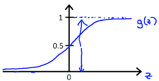
So based on the hypothesis, we will predict y=1 if ( J(\theta) ) >= 0.5. In other word, when ( \theta^\top x ) >= 0.
And that is called decision boundary.
The decision boundary can be non-linear when we use other function in ( \theta^\top x ) just like in linear regression.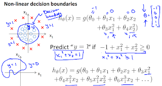
Then in cost function.
The cost function in linear regression is: ( J(\theta) = \frac{1}{2m} \sum{i=1}^m{(h{\theta}(x^{(i)}) - y^{(i)})^2} )
We cannot use it in logistic regression because the (h_\theta(x)) is change. And it contain a sigmoid function that it produces a non-convex function when we use this cost function.
Therefore, we change the function inside the summation to: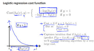
Because we use it in binary classification, and y=0 or 1, so can simplified it to: ( -ylog(h\theta(x))-(1-y)log(1-h\theta(x)) )
Finally the cost function is: ( J(\theta) = -\frac{1}{m}[\sum{i=1}^m{ y^{(i)} log(h\theta(x^{(i)})) + (1-y^{(i)}) log(1-h_\theta(x^{(i)})) }] )
And it is derived from statistics using the principle of maximum likelihood estimation. It also has a nice property that it is convex.
Now we have cost function, we can use it to do gradient descent to find the minimum cost. Same as in linear regression, the gradient descent is:
( \theta_j = \theta_j - \alpha \frac{\partial}{\partial\theta_j} J(\theta) )
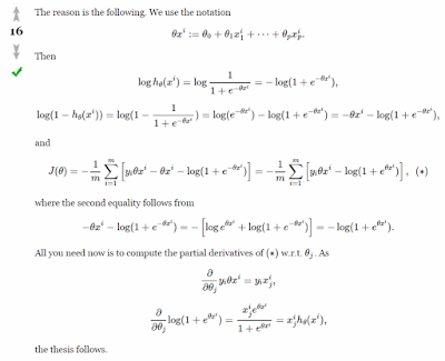
After differential the cost function, we can get:
( \theta_j = \thetaj - \alpha \frac{1}{m} \sum{i=1}^m{(h_{\theta}(x^{(i)}) - y^{(i)}) xj^{(i)}} )
In surprise, it’s totally same as the gradient descent in linear regression.
The way to differential the cost function is show in below by picture.
http://math.stackexchange.com/questions/477207/derivative-of-cost-function-for-logistic-regression
[](http://3.bp.blogspot.com/-kXLqV5SwoL4/VOtaMF-UGdI/AAAAAAAAANc/M8SEcFVYgo4/s1600/FireShot%2BCapture%2B-%2Bstatistics%2B-%2Bderivative%2Bof%2Bcost%2Bfunctio%2B-%2Bhttp_math.stackexchange.com_questi.png)
We can do gradient descent by vectorization in matlab:
In addition to gradient descent, there are other way to optimize the cost function. Like Conjugate gradient, BFGS, L-BFGS. The advantages are no need to select ( \alpha ) rate and more fast. But disadvantage is more complex.
However, we can use them easily by matlab without knowing any about their actually algorithm.
What we need to do in matlab is writing the function return cost and the partial derivatives value when given theta. And matlab will chose the appropriate method for us.
For example, the function we should write in the format like:
function [jVal, gradient] = costFunction(theta)And use it by:
jVal = (theta(1)-5)^2 + (theta(2)-5)^2;
gradient = zeros(2,1);
gradient(1) = 2(theta(1)-5);
gradient(2) = 2(theta(2)-5);
options = optimset(‘GradObj’, ‘on’, ‘MaxIter’, ‘100’);The optTheta will be the optimization theta.
initialTheta = zeros(2,1);
[optTheta, functionVal, exitFlag] = fminunc(@costFunction, initialTheta, options);
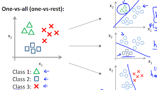
Besides, we can also use logistic regression in multi-calss classification.
The way is just train a logistic regression classifier for each class. And pick the class that probability is maximum as the result.
